Chapter: 6 The Star Schema: The Backbone of Analytical Models
Reliable analytics do not start with visuals or calculations. They start with structure.
In Power BI, the structure that gives you clarity, consistency, and trust is the star schema. It is not a Power BI feature. It is a data modeling pattern from data warehousing, described in detail by Kimball and Ross in The Data Warehouse Toolkit, and Microsoft’s own guidance recommends it for Power BI models.
In this chapter you will connect the five cleaned tables from Chapter 5 into a star schema, and check that it works.
6.1 Facts and Dimensions
A star schema classifies every table as one of two types.
Dimension tables describe the things you report on: patients, facilities, places, and time. Each row is one thing, identified by a unique key. Dimension columns are used to filter and group.
Fact tables record events or observations: visits, tests, targets. Each row is one event. A fact table contains the keys of the dimensions that describe the event, plus the values you summarize.
| Table | Type | One row is… | Key |
|---|---|---|---|
fact_patient_visits |
Fact | one patient visit | visit_id |
fact_targets |
Fact | one target for one facility, quarter and indicator | – |
dim_patient |
Dimension | one patient | patient_id |
dim_facility |
Dimension | one facility | facility_id |
dim_date |
Dimension | one calendar day | date_id |
The fact tables sit in the centre; the dimension tables surround them. Drawn out, the relationships form a star.
6.1.1 Why facts should not carry descriptions
It is tempting to copy facility names, districts or month names into the visit table “to make things simpler”. This creates three problems:
- Redundancy: the same description is stored on thousands of rows.
- Inconsistency: when a description changes, old and new rows disagree.
- Fragility: every report that used the copied column must be fixed.
That is why you removed year, quarter, month and iso_week from
the fact tables in Chapter 5. The fact table keeps only
date_id; everything about the date lives in dim_date.
6.1.2 Keys connect; they do not describe
A good key:
- uniquely identifies one row in its dimension,
- does not change over time,
- has no meaning of its own.
patient_id, facility_id and date_id are good keys. Names and labels
are bad keys: they change, they are misspelled, and they are not always
unique. In this dataset, for example, the same district name appears in
more than one state (see the data dictionary), so
district could never identify a place on its own.
6.1.3 Grain: what one row represents
The grain of a fact table is what one row represents.
fact_patient_visits has a daily grain: each row has the date of
the visit. fact_targets has a quarterly grain: each target applies
to a whole quarter, and its date_id holds the first day of that
quarter (for example 20240401 for Q2).
Microsoft’s guidance recommends exactly this approach for facts stored at a higher grain than the date table: store the first date of the period and create a normal one-to-many relationship. You will see in Step 10 what happens when such a table is viewed by month, and Chapter 7 shows how to handle it.
6.2 Relationships and Filter Direction
A relationship tells Power BI how a filter on one table reaches another. In a star schema, every relationship is:
- One-to-many (shown in Power BI as Many to one (*:1) when you start from the fact table): one patient has many visits; one facility has many visits; one date has many visits.
- Single direction: filters flow from the dimension (the “one” side) to the fact (the “many” side). Selecting a state limits the visits; selecting a month limits the visits.
Our model has two fact tables that share dim_facility and dim_date.
Microsoft’s documentation specifically advises against setting cross
filter direction to Both in this situation, a pattern it describes
using sales and budget tables that share lookup tables. Visits and
targets are the same pattern. Keep every relationship Single.
6.3 Hands-On: Building the Model
Work through these steps in order.
6.3.1 Step 1: Switch Off Two Automatic Features
Power BI Desktop does two things automatically that work against a deliberate model.
Auto date/time creates a hidden date table for every date column.
These hidden tables cannot be seen in the Data pane or Model view, and
they compete with dim_date.
Autodetect relationships creates relationships by matching column names after data is loaded. You want to create and check each relationship yourself.
- Select File → Options and settings → Options.
- Under Current File, select Data Load.
- In the Time intelligence section, clear Auto date/time.
- In the Relationships section, clear Autodetect new relationships after data is loaded.
- Select OK.
To change these settings for all new files too, make the same changes under Global → Data Load.
6.3.2 Step 2: Remove Any Relationships Created Automatically
- Select the Model view icon in the left sidebar.
- If any lines already connect your tables, select each line and press Delete, then confirm.
You should now see five unconnected tables.
6.3.3 Step 3: Create the Relationships
Create these five relationships. In Model view, drag the key column from the fact table and drop it on the matching column in the dimension table.
| From (many side) | To (one side) |
|---|---|
fact_patient_visits[patient_id] |
dim_patient[patient_id] |
fact_patient_visits[facility_id] |
dim_facility[facility_id] |
fact_patient_visits[date_id] |
dim_date[date_id] |
fact_targets[facility_id] |
dim_facility[facility_id] |
fact_targets[date_id] |
dim_date[date_id] |
For each relationship, check its settings. Select the line and look at the Properties pane, or double-click the line to open the relationship editor:
- Cardinality: Many to one (*:1)
- Cross-filter direction: Single
- Make this relationship active: Yes
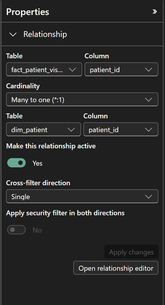
If Power BI offers Many to many instead, stop. It means the dimension column contains duplicate values. Go back to Power Query and check the dimension table: a key column must be unique.
6.3.4 Step 4: Arrange the Tables as a Star
Drag the tables so that the two fact tables are in the middle and the three dimension tables are around them. No dimension table should be connected to another dimension table.
This layout is not decoration. When something goes wrong, you can see at a glance which table filters which.
6.3.5 Step 5: Mark dim_date as the Date Table
Power BI needs to know which table is your calendar. Microsoft’s
documentation states that you must mark a date table when its
relationships use a column that is not a date, such as a whole-number
key like 20241231. Our relationships use date_id, so this step is
required for the time calculations in Chapter 7.
- In the Data pane, right-click
dim_date. - Select Mark as date table → Mark as date table.
- Choose the
datecolumn and confirm.
Power BI checks that date has unique values, no blanks, and no gaps
between the first and last date. dim_date has one row for every day of
2024, so the check passes.
6.3.6 Step 6: Sort Months in Calendar Order
Text sorts alphabetically, so months would appear as Apr, Aug, Dec, Feb…
Use month_num to sort them.
- Switch to Report view. (The Sort by Column command is on the Column tools tab, which Microsoft’s documentation says to use from Report view.)
- In the Data pane, select
dim_date[month]. - On the Column tools tab, select Sort by column → month_num.
This works because each month name has exactly one month number. A sort-by column must have one value for each value of the column being sorted.
quarter (Q1–Q4) already sorts correctly as text.
6.3.7 Step 7: Add the ART Start Date as an Inactive Relationship
fact_patient_visits contains a second date: art_start_date. To count
ART initiations by month, the date table must be able to filter that
column too.
Only one relationship between two tables can be active. The active
one (via date_id) filters visits by visit date. A second relationship
must be inactive; it is used only when a DAX measure asks for it
with the USERELATIONSHIP function (Chapter 7).
- In Model view, drag
fact_patient_visits[art_start_date]ontodim_date[date]. - Power BI creates the relationship as inactive, because an active relationship already exists between these tables. It appears as a dashed line.
- Check: Many to one (*:1), Single, not active.
Why not tb_test_date as well? A date table must contain every date
you relate to it. 18 TB test dates fall in January 2025, outside
dim_date. To analyse TB tests by test date, you would first extend
dim_date.
6.3.8 Step 8: Build Hierarchies
A hierarchy lets users drill down from summary to detail in a visual.
Date hierarchy:
- In the Data pane, right-click
dim_date[year]and select Create hierarchy. - Add
quarter,monthanddateto the hierarchy, in that order. - Rename the hierarchy
Calendar.
Location hierarchy: repeat with dim_facility[state], then
district, then facility_name. Name it Location.
In a hierarchy, District 3 under State A and District 3 under
State B are shown as separate rows, which is correct. But a slicer or
chart that uses district on its own combines them. In this dataset,
always use district together with state.
6.3.9 Step 9: Hide Keys and Technical Columns
Keys are essential for relationships but meaningless to report users.
Hiding them prevents accidental misuse, such as summing facility_id.
In the Data pane, right-click each field below and select Hide:
-
fact_patient_visits:visit_id,patient_id,facility_id,date_id -
fact_targets:facility_id,date_id -
dim_patient[patient_id],dim_facility[facility_id],dim_date[date_id],dim_date[month_num]
Hidden columns still work in relationships and DAX. In Table view, they appear greyed out.
6.4 Step 10: Validate the Model
Before writing indicators, prove that filters flow as expected. You need two simple measures. Chapter 7 explains measures properly; for now, create them as follows:
- Select
fact_patient_visitsin the Data pane. - On the Home tab, select New measure and enter:
Total Visits = COUNTROWS ( fact_patient_visits )- Select
fact_targets, select New measure, and enter:
Total Target = SUM ( fact_targets[target] )6.4.1 Test 1: Filtering by state
Create a Table visual with dim_facility[state], Total Visits and
Total Target.
| state | Total Visits | Total Target |
|---|---|---|
| State A | 4,483 | 9,321 |
| State B | 3,064 | 6,325 |
| State C | 2,453 | 5,116 |
| Total | 10,000 | 20,762 |
If every row shows the same number as the total, that measure’s table is
not connected to dim_facility. Check the relationship in Model view.
6.4.2 Test 2: Filtering by quarter
Replace state with dim_date[quarter].
| quarter | Total Visits | Total Target |
|---|---|---|
| Q1 | 2,456 | 5,179 |
| Q2 | 2,489 | 5,157 |
| Q3 | 2,524 | 5,210 |
| Q4 | 2,531 | 5,216 |
Both fact tables respond to the same date filter. This is the shared dimension at work.
6.4.3 Test 3: Filtering by month (and the grain problem)
Replace quarter with dim_date[month].
- Total Visits shows a value for every month, from Jan (846) to Dec (835), in calendar order. If the months are in alphabetical order, revisit Step 6.
- Total Target shows values only for Jan, Apr, Jul and Oct, which are the quarter totals. Every other month is blank.
This is not a bug. Targets are stored on the first day of each quarter, so the January row receives the whole Q1 target. Microsoft’s guidance describes this exact behaviour for higher-grain facts and recommends controlling it with a measure that returns blank below the quarter level. You will write that measure in Chapter 7. Until then, never show targets by month or by day.
6.5 Common Modeling Errors
Most broken models do not fail loudly. Numbers still appear and charts still render, but the logic underneath is wrong.
6.5.1 1. Many-to-many relationships created by accident
How it happens: a dimension table has duplicate keys; two fact tables are joined directly; text labels are used as keys; a summary table is joined to a line list on a non-unique column.
Why it is dangerous: totals can be inflated or vary depending on the visual.
What to do: relate fact tables only through shared dimensions, as
fact_patient_visits and fact_targets share dim_facility and
dim_date. Microsoft’s guidance generally recommends against relating
two fact tables directly. If a dimension has duplicate keys, fix it in
Power Query.
6.5.2 2. Bi-directional filters used to “fix” a visual
How it happens: a slicer does not behave as expected, and setting cross-filter direction to Both seems to solve it.
Why it is dangerous: filters travel along paths you did not intend, and results change with the layout of the report. With two fact tables sharing dimensions, as here, it creates ambiguity.
What to do: keep relationships Single. If you need a filter to reach a table it cannot reach, the structure is usually missing a dimension; fix the structure first.
6.5.3 3. Descriptions used as keys
How it happens: names are readable and available in every file, so they get used to join tables.
Why it is dangerous: names change, are misspelled, and are not
always unique. In this dataset, district alone would join facilities
from different states.
What to do: use stable identifiers. Keep descriptions in dimension tables.
6.5.4 4. Dimension tables linked to each other
How it happens: two dimensions share an attribute, so they get connected “to help” Power BI.
Why it is dangerous: there is more than one path between tables, and results depend on which path Power BI uses.
What to do: connect dimensions only to fact tables. If two dimensions need to interact (for example, patients and facilities), they do so through the events that connect them: the visits.
6.6 A Simple Rule to Remember
If your model is hard to explain, needs frequent filter overrides, produces inconsistent totals, or breaks when visuals change, the problem is rarely DAX. It is almost always the model.
Strong models make analytics boring. Weak models make analytics confusing.
6.7 Stop Point: Before You Write Indicators
Confirm that:
- Auto date/time and relationship autodetect are off for this file.
- There are exactly five active relationships, all Many to one and Single, from the fact tables to the dimension tables.
- There is one inactive relationship, from
art_start_datetodim_date[date]. - No dimension table is connected to another dimension table.
-
dim_dateis marked as the date table, using thedatecolumn. -
monthsorts bymonth_num. - Keys are hidden.
- Tests 1 to 3 give the numbers shown above.
If any of these is not true, fix it now.
6.8 What Comes Next
With a star schema in place, Power BI can:
- apply every slicer consistently to both fact tables,
- filter by visit date or, when asked, by ART start date,
- support indicator definitions that are written once and trusted everywhere.
The next chapter introduces DAX measures, where numerators and denominators are defined once and reused everywhere.
A strong model makes DAX simpler. A weak model makes DAX fragile.
Power BI for M&E and Public Health Data Analysts · The Growing Analyst